The 2019 explosions of Stromboli

Visiting an active volcano is a breathtaking experience and each year thousands of tourists around the world are seeking out the thrill to experience the power of the restless earth. One of the most visited active volcanoes in the world is Stromboli, a volcano known as the “Lighthouse of the Mediterranean” on a small island of the same name just off the coast of Sicily. Its persistent explosive Strombolian activity consists of several hundred of small eruptions per day. Visiting this fiery mountain (that allegedly J. R. R. Tolkien identified with his fictional volcano Mount Doom in the Lord of the Rings) comes at a certain risk though – on very rare occasions it produces major explosions, when as a tourist you might want to be as far away as possible from this island. To protect the tourists and the inhabitants of the island, the Italian National Institute for Geology and Volcanology (INGV) has installed a network that measures the seismic activity of Stromboli volcano and constantly monitors various parameters that characterize its state. Every morning the INGV researchers have a briefing with the local government and if the volcano shows anomalous behavior they can suspend the possibility to access the top of the volcano.

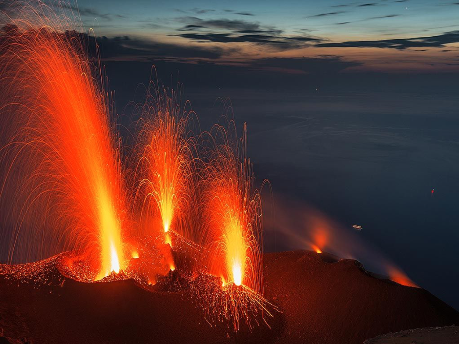
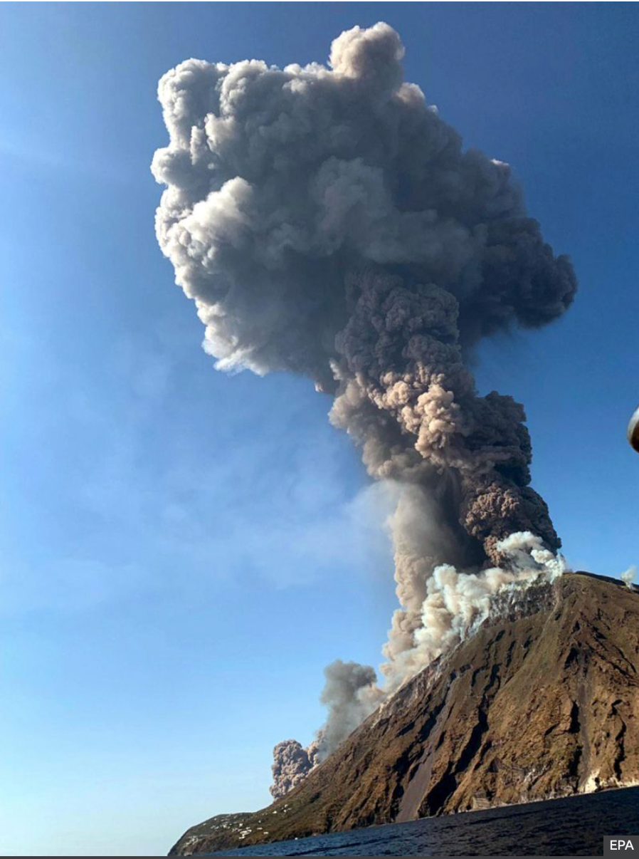
Figure 1: The left panel shows a typical Strombolian explosion that occurs several times per day. The right panel displays a snapshot of the major explosion on July 3.

Despite all of these measures, Stromboli erupted on the 3rd of July 2019 without showing any anomaly in the routinely monitored parameters. The explosion caused a pyroclastic flow (a fast-moving current of hot gas and volcanic matter) that extended for several hundred meters into the sea. Unfortunately, the event also claimed one fatality and could have been much worse and lead to a catastrophe if it had occurred a few hours later in the evening when many people climb the volcano in guided groups. On the 28th of August 2019 a second paroxysm occurred similar to that of July 3 with another pyroclastic flow, luckily this time without any fatalities.

The quest for predictive parameters

Since the routinely monitored seismic parameters did not predict this major eruption, the researchers of the INGV are now analyzing the collected seismic data in order to understand whether other seismic parameters showed any anomalies in the months prior to the 2019 eruptions. Ideally one wants to find new parameters that potentially can predict major eruptions in the future to make the experience of visiting Stromboli safer for future tourists and inhabitants. A major challenge is hereby that the 2019 explosions are the first measurements of such strength at Stromboli – the previous one occurred in 2002 when the network was not installed yet. Therefore at the moment it is impossible to quantify whether possible anomalies in the seismic parameters are indeed able to predict a major explosion – only the future will tell.

Within the context of my secondment at the INGV in Naples I had the possibility to work with the INGV seismologists to explore new seismic parameters by making use of unsupervised Machine Learning. In the past it had been conjectured that there is a connection between the waveforms of the seismic signals that are associated with the daily occurring Strombolian explosions (see left panel of Figure 1) and the physical state of the volcano, e.g. the gas mixture. Therefore we carried out a cluster analysis of the waveforms of the seismic signals to study how different clusters of waveforms behave in the time period of the 2019 paroxysms.

Visualization of seismic signals

In the period from May 2019 to September 2019 the INGV recorded around 20.000 seismic events that stem from the daily Strombolian explosions of the volcano. An example for a single signal is shown in Figure 2 below. The seismic signals that are associated with the explosions can be interpreted as time-series. In order to clean the signals, they are preprocessed by applying a band-pass filter that only allows frequencies between 0.05 – 0.5 Hz and the signals are downsampled to reduce the dimensionality of the time-series.

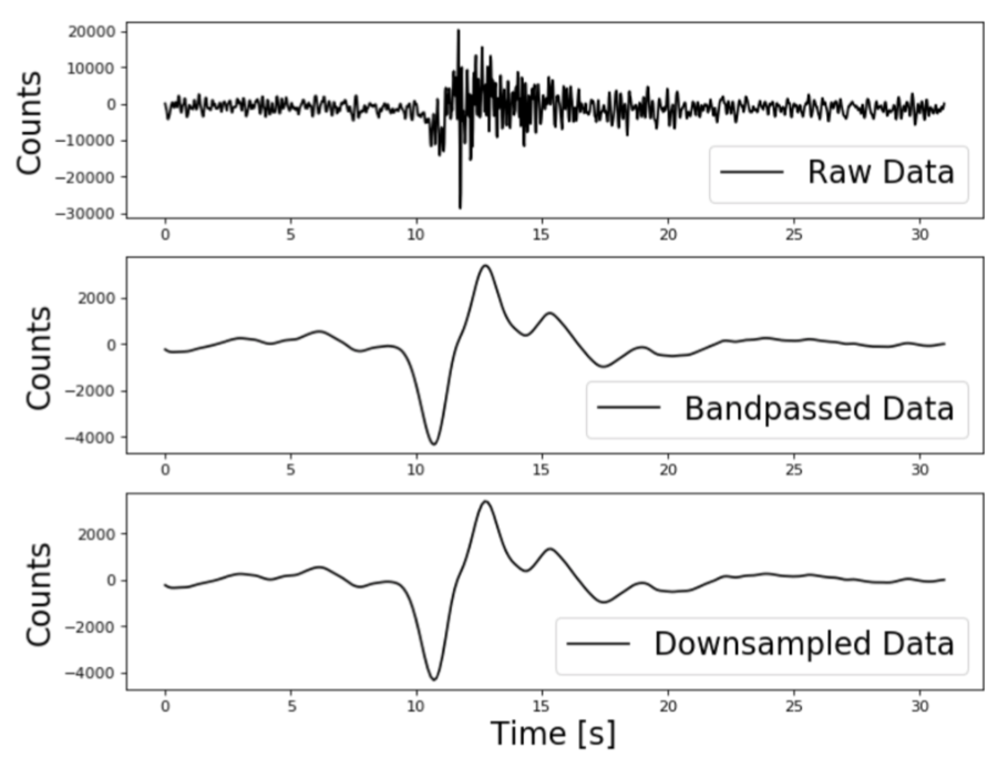
Figure 2: The left panel shows a seismic signal of a Strombolian explosion; the top panel shows the raw signal, the middle panel shows the same signal after applying a bandpass filter and the bottom panel shows the downsampled signal. The right panel shows the output of the t-SNE algorithm.

In data science several algorithms to visualize high dimensional data are available. In our case we use the t-SNE algorithm that allows to embed high dimensional data in a low dimensional space. Specifically, it models each high-dimensional object, in our case a high dimensional signal, by a two dimensional point in such a way that similar objects are modeled by nearby points and dissimilar objects are modeled by distant points with high probability. As such, t-SNE can be used to visualize clusters in the high-dimensional data. Running this algorithm with our dataset of seismic signals produces a 2D distribution that is shown in the right panel of Figure 2 above. Each of the displayed points corresponds to a high dimensional signal and it becomes visible that there are structures in the data that we can exploit with a clustering algorithm.

Clustering of seismic signals

Clustering defines structures by separating unlabeled datasets into homogeneous groups. For our analysis we use the K-Means algorithm which clusters data by trying to separate samples groups of equal variance, minimizing a criterion called within-cluster sum-of-squares. One of the challenges using K-Means is that the number of clusters has to be specified beforehand. Since we are working with unlabeled data, we don’t know the optimal number of clusters and there is no ground truth that could help us to assess the performance of our clustering. Thus the performance has to be evaluated using the model itself. One way to do so is to use Silhouette scores, that measure the separation distance between the resulting clusters. Higher scores relate to a model with better defined clusters. The Silhouette coefficient is calculated using the mean distance between a sample and all other points in the same class (a) and the distance between a sample and the nearest cluster that the sample is not a part of (b). The Silhouette coefficient for a single sample is then calculated as: (b - a) / max(a, b).

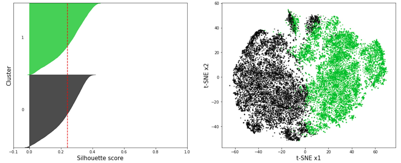
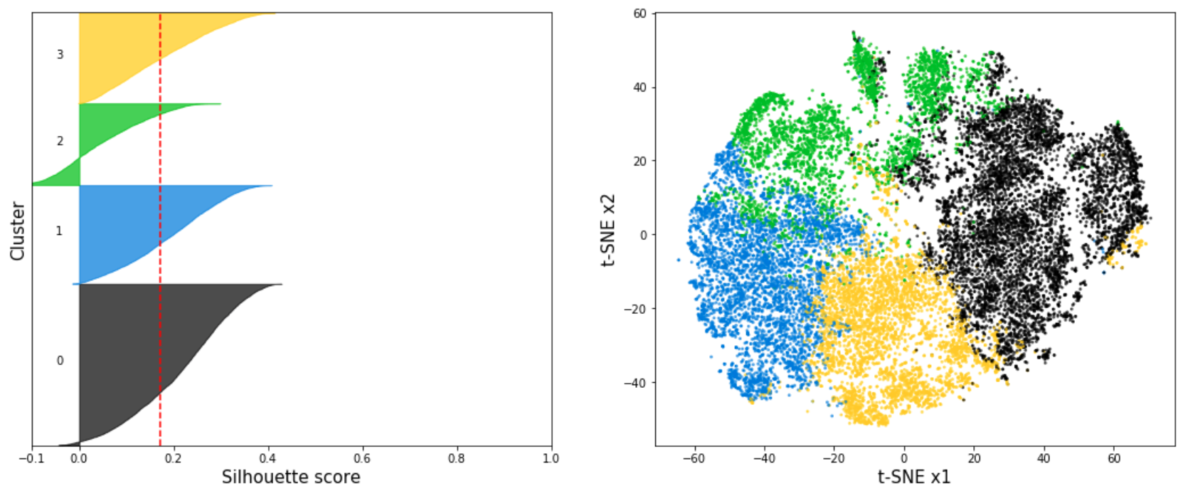
Figure 3: The top panel displays the Silhouette coefficients (left) and t-SNE projection (right) for K-Means with n=2 clusters. The bottom panel shows the Silhouette coefficients (left) and t-SNE projection (right) for K-Means with n=4 clusters.

Silhouette coefficients near +1 indicate that the sample is far away from the neighboring clusters. A value of 0 indicates that the sample is on or very close to the decision boundary between two neighboring clusters and negative values indicate that those samples might have been assigned to the wrong cluster.

In Figure 3 the silhouette coefficients and the t-SNE projection of the resulting clusters is shown for the K-Means algorithm with n=2 and n=4 clusters for the seismic signals associated with Strombolian explosions. The red line indicates the average silhouette score of all samples. In our analysis we found that the highest average silhouette score is obtained with n=2 clusters which indicates that the seismic signals form two main clusters. In Figure 4 the centroids of the two main clusters are shown. As expected, the waveforms of the two cluster centroids are very different. The example signal shown in Figure 2 can be clearly associated with Cluster 1.

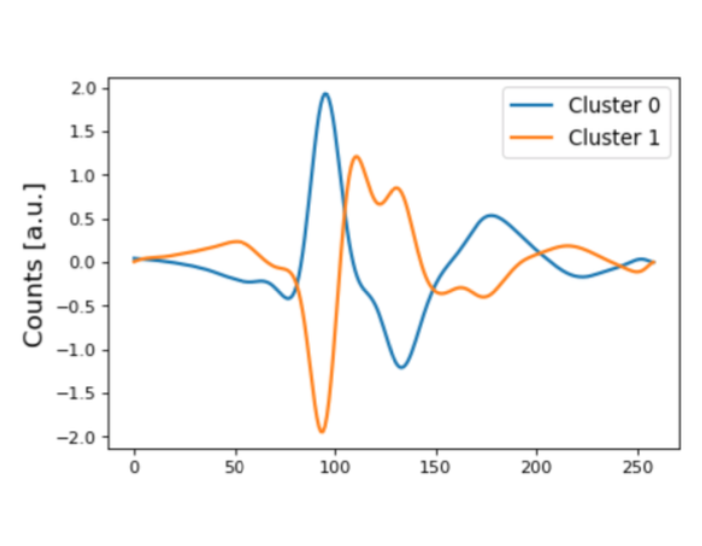
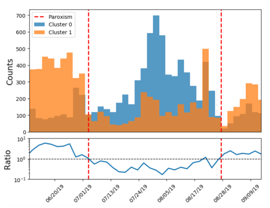
Figure 4: The left panel shows the centroids of the two main clusters obtained with the K-Means algorithm. The right panel shows the time evolution of the two main clusters.

Since we have access to the time stamps of the signals we can display the time evolution of the signals in the two main clusters. The resulting distribution from May 2019 to September 2019 is shown in the right panel of Figure 4 and the 2019 explosions are marked with red lines. We observe a strong asymmetry between the two clusters in this time period.

Conclusions

The researchers of the INGV conjecture that there is a connection between the waveforms of the signals associated to the Strombolian explosions and the physical state of the volcano. The observed asymmetry in the time evolution of the waveform clusters might therefore indicate large changes of the physical state of the volcano in the eruption period. The ratio between the two main waveform clusters might be an important variable to monitor the state of the volcano. In principle this variable can be monitored in real time by automatically assigning selected signals to one of the two clusters. The next important steps that the INGV researchers will take is analyzing the waveforms of the seismic signals for larger time scales and at the same time analyze controlled experiments set up in a laboratory to better understand the connection between the physical state of volcanic systems and the resulting seismic signals.

Moreover, given that most of the routinely monitored seismic parameters showed no anomaly prior to the major eruptions in 2019, the ratio of the two main waveform clusters may be potentially important to predict future explosions. However, as data analysts we are in a dilemma – on the one hand we need more data to understand which variables are correlated with major explosions of Stromboli – on the other hand we don’t want to hope for further major explosions that endanger the life of tourists and inhabitants. All that we can do is wait what the nature will bring us while trying our best to make use of the limited data we have to make visiting Stromboli a safe experience.